시작하기 전에 R, RStudio, KoNLP(한글 형태소 분석 패키지)가 설치되어 있어야한다.
특히 KoNLP는 다운받는 과정이 조금 복잡하므로 아래 링크를 참고하시길!
1. [R 프로그래밍] R, R Studio 다운로드
https://blog.naver.com/song_sec/221799018628
2. [R 프로그래밍] install.packages("KoNLP") - Konlpy 설치불가 이슈 해결
https://blog.naver.com/song_sec/221800340719
이번 포스팅에서는 R을 이용하여 카카오톡 채팅방을 아래 카테고리에 따라 분석할 것이다.
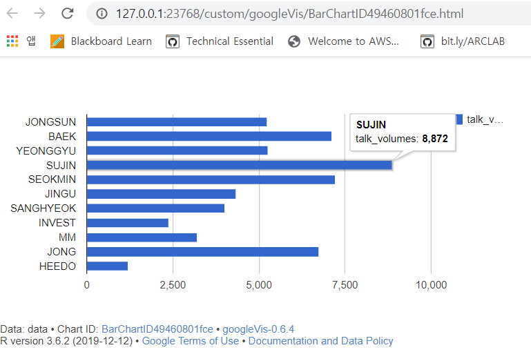
1) 카카오톡 채팅방에서 각 인원의 대화 지분
2) 시간대별 메세지 수 (몇시가 가장 활발하고, 몇시가 채팅이 없는지)
3) 가장 많이 등장하는 메세지(단어, 형태소) - 워드클라우드
4) 상관성 분석
나는 11명이 있는 친구들 단톡방을 대상으로 해당 분석들을 진행하였다.
1) 카카오톡 채팅방 각 인원의 대화 지분
(1) 결과물
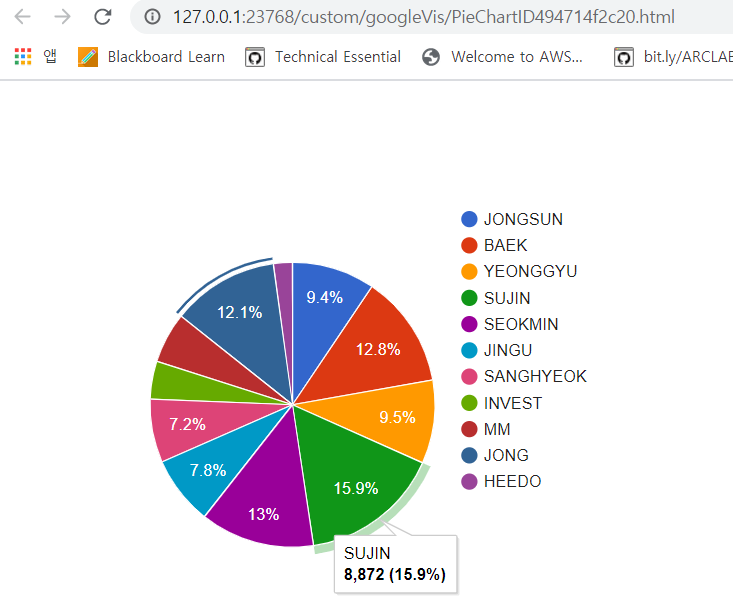
(2) 코드 설명

나는 카카오톡 대화내용을 받아온 후, 메모장에서 전체바꾸기로 각 사람들의 이름을 '[이름]'으로 변경했다. 이는 나중에 있을 텍스트분석에서 친구들이 말한 내이름, 내가 발언하여 생긴 내 이름과 분리 하기 위함이다.
하지만 이것은 R에서 str_replace_all을 통해 바꿀 수도 있으므로 참고만 하시길!
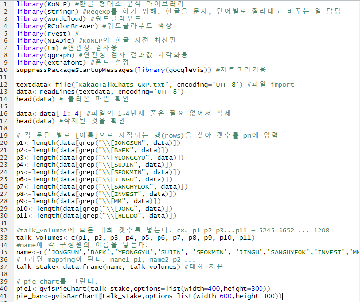
library(KoNLP) #한글형태소 분석 라이브러리
library(stringr) #Regexp를 하기 위해. 한글을 문자, 단어별로 잘라내고 바꾸는 일 담당
library(wordcloud) #워드클라우드
library(RColorBrewer) #워드클라우드 색상
library(rvest) #html, xml 자료를 쉽게 가져와서 처리
library(NIADic) #KoNLP의 한글 사전 최신판
library(tm) #연관성 검사용
library(qgraph) #연관성 검사 결과값 시각화용
library(extrafont) #폰트 설정
suppressPackageStartupMessages(library(googleVis)) #차트그리기용
textdata<-file("KakaoTalkChats_GRP.txt", encoding='UTF-8') #파일
import data<-readLines(textdata, encoding='UTF-8')
head(data) # 불러온 파일 확인 data<-data[-1:-4] #파일의 1~4번째 줄은 필요 없어서 삭제
head(data) #삭제된 것을 확인
# 각 문단 별로 [이름]으로 시작되는 행(rows)을 찾아 갯수를 pn에 입력
p1<-length(data[grep("\\[JONGSUN", data)])
p2<-length(data[grep("\\[BAEK", data)])
p3<-length(data[grep("\\[YEONGGYU", data)])
p4<-length(data[grep("\\[SUJIN", data)])
p5<-length(data[grep("\\[SEOKMIN", data)])
p6<-length(data[grep("\\[JINGU", data)])
p7<-length(data[grep("\\[SANGHYEOK", data)])
p8<-length(data[grep("\\[INVEST", data)])
p9<-length(data[grep("\\[MM", data)])
p10<-length(data[grep("\\[JONG", data)])
p11<-length(data[grep("\\[HEEDO", data)])
#talk_volumes에 모든 대화 갯수를 넣는다. ex. p1 p2 p3...p11 = 5245 5652 ... 1208 talk_volumes<-c(p1, p2, p3, p4, p5, p6, p7, p8, p9, p10, p11) #name에 각 구성원의 이름을 넣는다.
name<-c('JONGSUN','BAEK','YEONGGYU','SUJIN', 'SEOKMIN', 'JINGU','SANGHYEOK','INVEST','MM','JONG','HEEDO')
#그러면 mapping이 된다. name1-p1, name2-p2 ...
talk_stake<-data.frame(name, talk_volumes) #대화 지분 # pie chart를 그린다.
pie1<-gvisPieChart(talk_stake,options=list(width=400,height=300))
pie_bar<-gvisBarChart(talk_stake,options=list(width=600,height=300))
# 한글은 깨지는 경우가 있으므로 아래 코드를 추가한다.
header <-pie1$html$header header <- gsub("charset=utf-8", "charset=euc-kr", header)
pie1$html$header <- header #pieplot를 소환한다. plot(pie1) plot(pie_bar)
2) 시간대별 메세지 수 (몇시가 가장 활발, 몇시가 채팅이 없나)
(1) 결과물
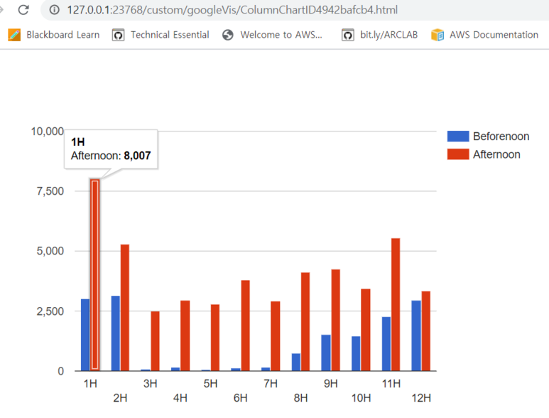
gvisColumnChart. 오후 1시 메세지가 가장 많았다.
(2) 코드 설명
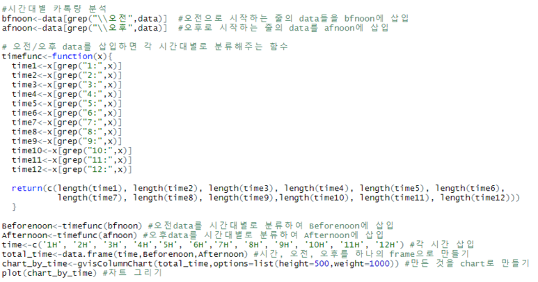
#시간대별 카톡량 분석
bfnoon<-data[grep("\\오전",data)] #오전으로 시작하는 줄의 data들을 bfnoon에 삽입
afnoon<-data[grep("\\오후",data)] #오후로 시작하는 줄의 data를 afnoon에 삽입
# 오전/오후 data를 삽입하면 각 시간대별로 분류해주는 함수
timefunc<-function(x){
time1<-x[grep("1:",x)]
time2<-x[grep("2:",x)]
time3<-x[grep("3:",x)]
time4<-x[grep("4:",x)]
time5<-x[grep("5:",x)]
time6<-x[grep("6:",x)]
time7<-x[grep("7:",x)]
time8<-x[grep("8:",x)]
time9<-x[grep("9:",x)]
time10<-x[grep("10:",x)]
time11<-x[grep("11:",x)]
time12<-x[grep("12:",x)]
return(c(length(time1), length(time2), length(time3), length(time4), length(time5), length(time6), length(time7), length(time8), length(time9),length(time10), length(time11), length(time12))) }
Beforenoon<-timefunc(bfnoon) #오전data를 시간대별로 분류하여 Beforenoon에 삽입
Afternoon<-timefunc(afnoon) #오후data를 시간대별로 분류하여 Afternoon에 삽입
time<-c('1H', '2H', '3H', '4H','5H', '6H','7H', '8H', '9H', '10H', '11H', '12H') #각 시간 삽입
total_time<-data.frame(time,Beforenoon,Afternoon) #시간, 오전, 오후를 하나의 frame으로 만들기
chart_by_time<-gvisColumnChart(total_time,options=list(height=500,weight=1000)) #만든 것을 chart로 만들기 plot(chart_by_time) #차트 그리기
3) 가장 많이 등장하는 메세지(단어, 형태소) 워드클라우드
(1) 결과물
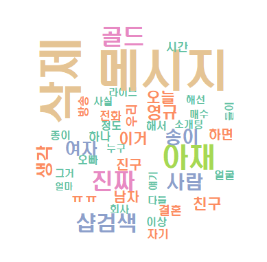
wordcloud. 놀랍게도 메세지 삭제를 애들이 많이해서 "삭제"가 제일 많다. ㅋㅋㅋㅋㅋㅋㅋㅋㅋㅋㅋㅋ
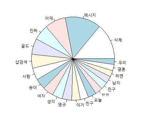
piechart
20대 11명 대화방에서 가장 많이 나오는 단어들 ㅋㅋㅋ
(2) 코드 설명
가. 데이터 전처리: 텍스트분석을 위해서는 필요없는 정보(시간, 특수문자 등)를 지우는 과정이 꼭 필요하다.
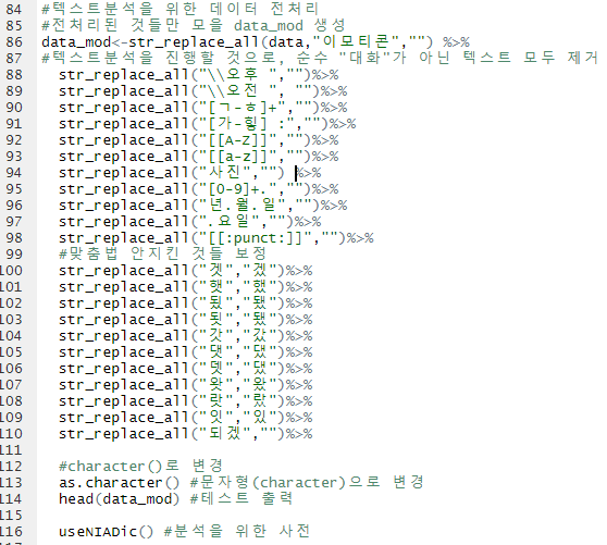
#텍스트분석을 위한 데이터 전처리 #전처리된 것들만 모을 data_mod 생성
data_mod<-str_replace_all(data,"이모티콘","") %>% #텍스트분석을 진행할 것으로, 순수 "대화"가 아닌 텍스트 모두 제거
str_replace_all("\\오후 ","")%>%
str_replace_all("\\오전 ", "")%>%
str_replace_all("[ㄱ-ㅎ]+","")%>%
str_replace_all("[가-힣] :","")%>%
str_replace_all("[[A-Z]]","")%>%
str_replace_all("[[a-z]]","")%>%
str_replace_all("사진","") %>%
str_replace_all("[0-9]+.","")%>%
str_replace_all("년.월.일","")%>%
str_replace_all(".요일","")%>%
str_replace_all("[[:punct:]]","")%>% #맞춤법 안지킨 것들 보정
str_replace_all("겟","겠")%>%
str_replace_all("햇","했")%>%
str_replace_all("됬","됐")%>%
str_replace_all("됫","됐")%>%
str_replace_all("갓","갔")%>%
str_replace_all("댓","댔")%>%
str_replace_all("뎃","댔")%>%
str_replace_all("왓","왔")%>%
str_replace_all("랏","랐")%>%
str_replace_all("잇","있")%>%
str_replace_all("되겠","")%>%
#character()로 변경
as.character() #문자형(character)으로 변경
head(data_mod) #테스트 출력
useNIADic() #분석을 위한 사전
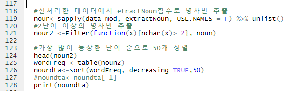
#전처리한 데이터에서 etractNoun함수로 명사만 추출
noun<-sapply(data_mod, extractNoun, USE.NAMES = F) %>%
unlist() #2단어 이상의 명사만 추출
noun2 <-Filter(function(x){nchar(x)>=2}, noun)
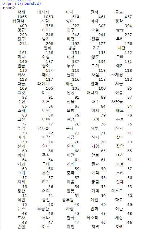
#가장 많이 등장한 단어 순으로 50개 정렬
head(noun2) wordFreq <-table(noun2)
noundta<-sort(wordFreq, decreasing=TRUE,50) #noundta<-noundta[-1]
print(noundta)
나. 워드클라우드 및 piechart
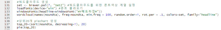
#워드클라우드 생성
set <- brewer.pal(7, "Set2") #워드클라우드를 위한 폰트색상 계열 설정
loadfonts(device="win") #폰트 불러오기
windowsFonts(headline=windowsFont("HY헤드라인M")) wordcloud(names(noundta), freq=noundta, min.freq = 100, random.order=T, rot.per = .1, colors=set, family="headline")
#상위20개 piechart 생성
top_20=(sort(noundta, decreasing=T), 20) pie(top_20)
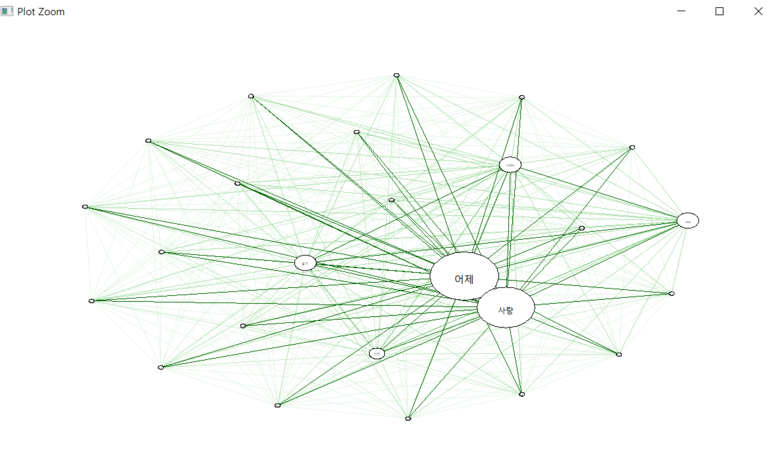
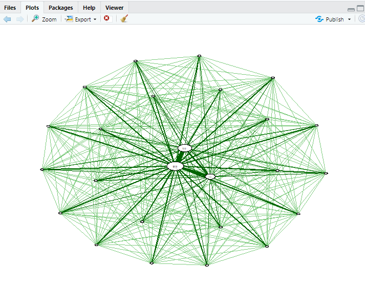
4) 상관성분석
(1) 결과물
(2) 코드설명
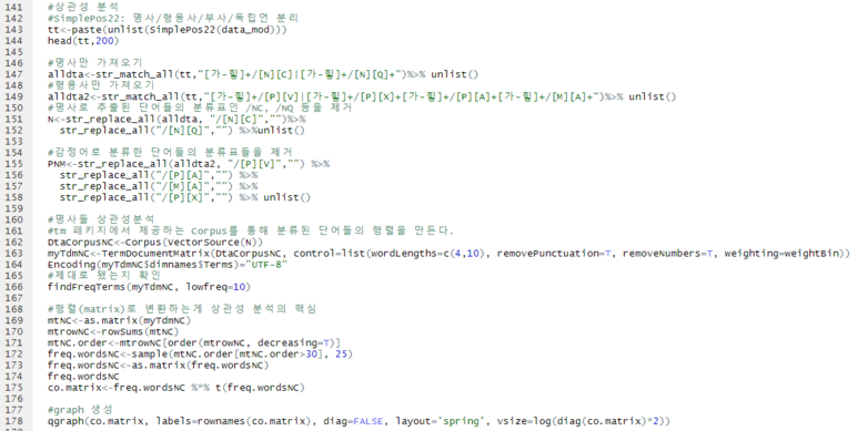
#상관성분석
#SimplePos22: 명사/형용사/부사/독립언 분리
tt<-paste(unlist(SimplePos22(data_mod)))
head(tt,200)
#명사만 가져오기
alldta<-str_match_all(tt,"[가-힣]+/[N][C]|[가-힣]+/[N][Q]+")%>%
unlist() #형용사만 가져오기
alldta2<-str_match_all(tt,"[가-힣]+/[P][V]|[가-힣]+/[P][X]+[가-힣]+/[P][A]+[가-힣]+/[M][A]+")%>%
unlist() #명사로 추출된 단어들의 분류표인 /NC, /NQ 등을 제거
N<-str_replace_all(alldta, "/[N][C]","")%>%
str_replace_all("/[N][Q]","") %>%unlist()
#감정어로 분류한 단어들의 분류표들을 제거
PNM<-str_replace_all(alldta2, "/[P][V]","") %>%
str_replace_all("/[P][A]","") %>%
str_replace_all("/[M][A]","") %>%
str_replace_all("/[P][X]","") %>% unlist()
#명사들 상관성분석 #tm 패키지에서 제공하는 Corpus를 통해 분류된 단어들의 행렬을 만든다.
DtaCorpusNC<-Corpus(VectorSource(N))
myTdmNC<-TermDocumentMatrix(DtaCorpusNC, control=list(wordLengths=c(4,10), removePunctuation=T, removeNumbers=T, weighting=weightBin)) Encoding(myTdmNC$dimnames$Terms)="UTF-8"
#제대로 됐는지 확인
findFreqTerms(myTdmNC, lowfreq=10)
#행렬(matrix)로 변환하는게 상관성 분석의 핵심
mtNC<-as.matrix(myTdmNC)
mtrowNC<-rowSums(mtNC)
mtNC.order<-mtrowNC[order(mtrowNC, decreasing=T)]
freq.wordsNC<-sample(mtNC.order[mtNC.order>30], 25)
freq.wordsNC<-as.matrix(freq.wordsNC)
freq.wordsNC co.matrix<-freq.wordsNC %*% t(freq.wordsNC) #graph 생성
qgraph(co.matrix, labels=rownames(co.matrix), diag=FALSE, layout='spring', vsize=log(diag(co.matrix)*2))
5) 형용사(감정어) 상관성분석
(1) 결과물
(2) 코드설명: 위의 4) 명사 상관성분석과 코드는 모두 동일하며 NC부분만 PNM으로 변경했다.
# 형용사(감정어) 상관성분석
DtaCorpusPNM<-Corpus(VectorSource(PNM))
myTdmPNM<-TermDocumentMatrix(DtaCorpusPNM, control=list(wordLengths=c(4,10), removePunctuation=T, removeNumbers=T, weighting=weightBin)) Encoding(myTdmPNM$dimnames$Terms)="UTF-8" findFreqTerms(myTdmPNM, lowfreq=10)
mtPNM<-as.matrix(myTdmPNM)
mtrowPNM<-rowSums(mtPNM)
mtPNM.order<-mtrowNC[order(mtrowPNM, decreasing=T)]
freq.wordsPNM<-sample(mtNC.order[mtPNM.order>30], 25)
freq.wordsPNM<-as.matrix(freq.wordsPNM)
freq.wordsPNM co.matrix<-freq.wordsPNM %*% t(freq.wordsPNM)
qgraph(co.matrix, labels=rownames(co.matrix), diag=FALSE, layout='spring', vsize=log(diag(co.matrix)*2))
4), 5)의 상관성분석은 아직 잘 이해가 안되어서 조금 더 공부해보아야할 것 같다.
그래도 R 1일차 치고 이정도면 만족스러운 결과물이다!!!
내가 R을 다운받게된 계기는 이 분석을 진행하기 위해서였는데, 코드의 출처는 아래 링크와 같다.
다만 2017년 게시글이다보니 저때와 지금의 카톡 내려받기 txt 포맷이 조금 달라서(어느 os에서 다운받느냐에 따라 또 다르다!!!) 나는 조금씩 수정 하며 진행한 점을 참고하면 되겠다.
내 코드는 안드로이드에서 다운받은 카카오톡 대화내용 기준이다!
(그래봤자 data검색 / replace format쪽만 수정하면 된다)
'직장생활 > Programming (C, Python)' 카테고리의 다른 글
| [R 프로그래밍] install.packages("KoNLP") - Konlpy 설치불가 이슈 해결 (0) | 2021.07.29 |
|---|---|
| [R 프로그래밍] Fail to install scala-library-2.11.8.jar. Recommand to install library manually in C:/User (0) | 2021.07.29 |
| [R 프로그래밍] R, R Studio 다운로드 (0) | 2021.07.29 |
| [R 프로그래밍] R Studio 설치/다운로드 (0) | 2021.07.29 |
| [Jupyter notebook] PyCharm보다 편한 주피터 노트북 1분만에 설치하기 (0) | 2021.07.29 |